TIGRE Telescope
Response curve

Menu:
Update:
16th January 2024
Response curve
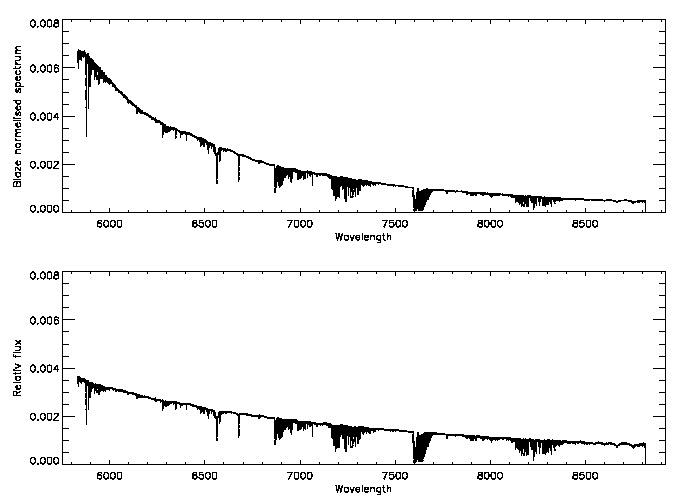
The main result of the pipeline is the blaze normalised spectrum. To correct the global trend and the small scale variations caused by the reduction, one can use a response curve. This response curve is estimated from a observed standard star with TIGRE telescope and a reference spectrum of this standard star (ref_spec). The used reference spectra are form the ESO database . To obtain the response curve, the telluric line are removed from the observed spectrum. In the next step, the observed spectrum are smooth and broadened (obs_spec_sb) and once only smooth (obs_spec_s). By the broadening the small scale variation are removed. To obtain the global response curve (resp_curve), the ratio of ref_spec and obs_spec_sb is calculated and can be written as:| resp_curve = ref_spec / obs_spec_sb. |
With this curve, one can correct the global trend and one obtains a relative flux because the reference spectrum is set on the level of the blaze normalised spectrum. To correct a spectrum, the response curve is multiply with the object spectrum (obj_spec). This can be written as:
| obj_spec_corr = obj_spec * resp_curve. |
In the figure, one can seen an example of this correction.
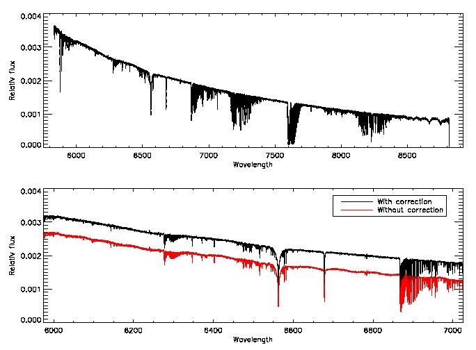
| frac = obs_spec_sb / obs_spec_s. |
The variation in the Hα, HHβ, Hγ and H&delta lines are interpolated from the variations before and after the line. To remove the small scale variations with this correction, one multiply this correction with the spectrum. This can be written as:
| obj_spec_corr = obj_spec * frac. |
In the figure, one can seen an example of this correction. In the upper plot, the total spectrum is shown. In the lower plot, the Hα is seen. The black curve is the corrected spectrum and the red is the spectrum without this correction. One can seen that the small scale variations are removed in the black curve.
Note: If no standard star was observed then the values for the global response curve and the small scale variations 1.